COPRA2 – Constructing Proxy Records From Age Models

Introduction

COPRA transforms dating (age–depth) uncertainties into proxy uncertainties. Given a set of dated depths with age errors and a proxy record measured along the same depth axis, it builds a Monte Carlo ensemble of age–depth models, interpolates the proxy onto each realisation, and reports the proxy time series with confidence bands. Every run records its random seed, so results are exactly reproducible.

The software offers two front ends over one shared computational core: a desktop application (copra-gui) and a command-line tool (copra-cli).

Installation

From PyPI (with pip) (not yet implemented)

The distribution name is copra2 (the name copra was already taken); the import package and the console commands keep the copra name:

pip install copra2      # then: copra-gui  /  copra-cli  /  import copra

From source (developers)

cd copra_py
python -m venv .venv
source .venv/bin/activate      # Windows: .venv\Scripts\activate
pip install -e ".[dev]"

Standalone application (end users)

A double-clickable application is built with PyInstaller and needs no Python installation:

pip install pyinstaller
pyinstaller packaging/copra.spec     # run from copra_py/

PyInstaller does not cross-compile; build on the target platform.

Launching the app

From a source checkout:

copra-gui                  # entry point
python -m copra.gui        # equivalent

Or double-click the standalone application built above.

Input data formats

Input files are plain whitespace- or comma-separated text (.txt / .csv) with no column headers (lines starting with # or % are treated as comments). Depths must be strictly increasing and unique — no duplicate depths, no NaN values.

Example dating table (depth in mm, age in yr, error in yr):

0     0      0
120   980    45
250   2010   60
...

With asymmetric errors (columns: depth, age, lower error, upper error):

1      50     12.5   20.5
112    207.9  20.4   19.4
...

Asymmetric errors are sampled with a two-piece (split) normal — the lower error sets the spread below the age, the upper error above — so the Monte Carlo ensemble reflects the asymmetry. There is no MATLAB equivalent for this input.

Proxy errors (optional)

By default no proxy error is assumed. Two independent sources can be added and are folded in when the proxy is resampled onto the age-certain axis:

• Value error — the optional third proxy column. Each proxy value is perturbed by a Gaussian of that 1σ width, widening the proxy confidence band.
• Distance (sample-size) error — set Sample size in the GUI (or --sample-size on the CLI), in the same unit as the depth column of the proxy/dating files (e.g. mm). A proxy sample integrates over that depth width, so its depth is treated as uniform within ± half the sample size; the age is read at the perturbed depth, adding an age (distance) uncertainty. The sample size is constant over the record. Neither error is present in the original MATLAB COPRA.

Desktop application

The window is split into a control panel (left), plot tabs (right) and a log/status area (bottom). Hover any input field for a tooltip.

1. Select inputs. Choose the dating table and proxy record (and optionally a layer-count file). As soon as both required files are set, the review plots are drawn automatically.
2. Set parameters. Number of Monte Carlo realisations, interpolation method, confidence-interval widths, an optional random seed, and the sample/proxy names (see Parameters).
3. Review and treat. Inspect flagged age reversals and hiatus candidates; apply treatment if needed (see below).
4. Run. The Monte Carlo model runs on a background thread with a progress bar; press Cancel to abort.
5. Export. Write the results, ensemble, session and log to a chosen folder (File → Export results, or the Export button).

Menus

• File — Open session and Save session read and write a JSON session (all inputs, parameters, treatment and the random seed), so a run can be restored or reproduced; Export results writes the output files; Quit.
• Settings → Preferences — appearance mode (system / light / dark) and default run parameters (MC realisations, interpolation, confidence intervals, output folder). They are stored between sessions; the parameters prefill the fields on startup and the theme is applied immediately.
• Help — open this documentation in the browser, or the project website.
• About — version, authors, citation and license (About COPRA), and the Qt version (About Qt).

Plot tabs

When a reversal or an automatic hiatus is detected, a warning line prefixed with ⚠️ appears in the log/status area at the bottom.

Reversals & hiatuses

An age reversal is a dating point whose age is out of order relative to its depth. COPRA classifies reversals as tractable (resolvable by widening the age error) or non-tractable (best removed). Treatment is declarative and stored in the session, so a run configured in the GUI remains reproducible.

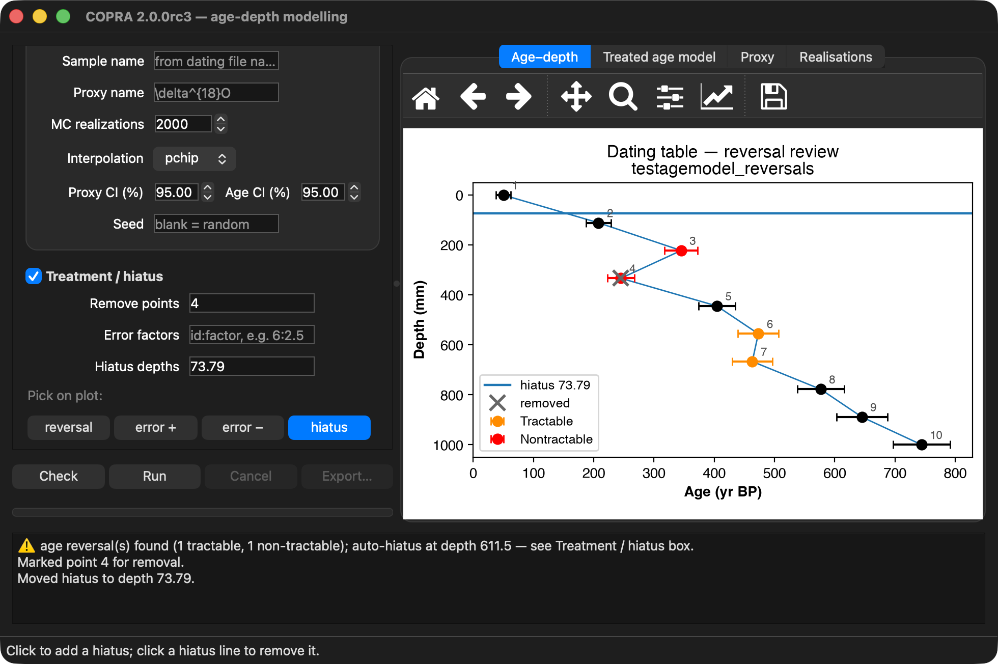
• Pick reversal — click a dating point to toggle its removal (struck-through when marked).
• Pick error increase / decrease — click a point to widen or narrow its age error on a 0.5 grid (1.5×, 2×, 2.5×, …). Widening a point can turn a non-tractable reversal tractable; its colour and error bar update immediately.
• Pick hiatus — on the Age–depth plot, click empty space to add a hiatus line, click a line to remove it, or drag a line to move it. A hiatus must lie strictly between two dating points.

All picking is done on the editable Age–depth plot; the Treated age model plot is the read-only result and is not interactive.

Automatic hiatus detection. COPRA flags gaps with an anomalously low growth rate as hiatuses. When one is found, its depth is written into the Hiatus depths field and drawn as a line on the Age–depth plot (and shown on the treated model); when none is found the field stays empty and no line is shown. Editing or clearing the field overrides the automatic value (auto-fill then stops). Note that an age reversal also produces a low-growth-rate gap, so a reversal can raise a spurious hiatus — treating the reversal removes it automatically.

Reusing an age model for another proxy

A single Monte Carlo age model can be applied to several proxy records measured on the same core without re-running the (expensive) simulation. After a run, load a different proxy file in the proxy picker: the Run button changes to Transfer. Clicking it (or using File → Replace proxy record) evaluates the computed age–depth realisations at the new proxy's depths (linear interpolation per realisation) and updates the Proxy and Realisations tabs immediately; the age model itself is unchanged.

The new proxy should cover the same depth range; depths outside the age model's range are dropped. To keep the original results safe, COPRA renames the sample (appending the new proxy's file name) and requires a new sample name when you export, so nothing is overwritten. Start a completely fresh project with File → Close.

Command line

The copra-cli command drives the same pipeline without a GUI.

# Guided, interactive session (prompts for files, parameters, treatment)
copra-cli interactive          # or just: copra-cli

# Inspect a dataset: reversals + hiatus candidates, no simulation
copra-cli check --dating DATING.txt --proxy PROXY.txt

# Run the age model and write outputs (+ optional plots)
copra-cli run --dating DATING.txt --proxy PROXY.txt \
    --M 2000 --interp pchip --seed 42 --output-dir output --plots

# Reversal treatment: remove point 3, widen point 6's error three times
copra-cli run --dating DATING.txt --proxy PROXY.txt \
    --remove-points 3 --increase-error 6 6 6

# Layer counting and an explicit hiatus depth
copra-cli run --dating DATING.txt --proxy PROXY.txt \
    --layercount LAYERS.txt --hiatus 389.5

# Reproduce a previous run exactly from its saved session
copra-cli reproduce output/d_<sample>_<date>.json

Options may also be supplied through a TOML file via --config run.toml (a [copra] table with the same keys); explicit command-line options override the file.

Output files

Each run writes four files. Names carry the sample name and the run date in ISO YYYY-MM-DD form.

Reproducibility

The JSON session is the authoritative record of a run. It stores the input file paths, all parameters and the resolved random seed. Feeding it back reruns the model to a bit-identical ensemble:

copra-cli reproduce output/d_sample_2026-09-13.json

If no seed is given, COPRA generates one and records it, so even “random” runs remain reproducible after the fact.

Parameters

Python API

The scientific core is a plain NumPy/SciPy package with no Qt or matplotlib dependency and can be scripted directly:

from copra.core.model import CopraSession
from copra.core.logging_ import run_session, save_results

session = CopraSession(
    dating_path="DATING.txt",
    proxy_path="PROXY.txt",
    M=2000,
    interp_method="pchip",
    samplename="mycore",
    seed=42,
)
run_session(session)                       # populates the ensemble + statistics
save_results(session, "output")            # writes the four output files

Package layout: copra.core (computation), copra.plotting (matplotlib figures), copra.gui (Qt6 application), copra.cli (command-line tool).

References

Breitenbach, S. F. M., Rehfeld, K., Goswami, B., Baldini, J. U. L., Ridley, H. E., Kennett, D. J., Prufer, K. M., Aquino, V. V., Asmerom, Y., Polyak, V. J., Cheng, H., Kurths, J., and Marwan, N. (2012): COnstructing Proxy Records from Age models (COPRA), Climate of the Past, 8, 1765–1779. doi:10.5194/cp-8-1765-2012

Project website: https://tocsy.pik-potsdam.de/copra2.php

Authors: Norbert Marwan and Sebastian F. M. Breitenbach (original and Python port).
Acknowledgements (original version): Kira Rehfeld, Bedartha Goswami, Daniel Juncu.