The first application of the ACE algorithm of Breiman and
Friedman (1985) in nonlinear dynamics.
This programme performs a calculation of optimal transformations
from a data set.
The algorithm has been invented by Breiman and Friedman (1985)
and the program follows it closely, besides two differences:
The output is not normalized with respect to the mean values of the
optimal transformations, so the mean values may not necessarily be zero.
The data are rank ordered before the calculation of the optimal
transformations. This leads to a simpler computation of
conditional expectation values.
The algorithm (but not the particular subroutine of estimating the
conditional expectation values) is also described in
Voss and Kurths (1997), Voss et al. (1999), Voss and Kurths (1999).
A comfortable clone of this programme can be found in the
CRP toolbox.
Usage
The procedure is defined as
function [psi,phi]=ace(x,ll,dim,wl,oi,ii,ocrit,icrit,shol,shil)
Therefore, the outputs are psi (the maximal correlation)
and phi (the set of optimal transformations).
There is another program, ace_m.m, that calls ace.m.
It can also be used to understand how ace.m has to be used.
The input parameters are defined as follows:
x
The data set of size (dim+1)×ll.
ll
The number of data points of each of the dim+1 terms, e.g. 1000, if the
regression analysis is performed on 1000 data tuples.
dim
The number of terms for the rhs, can be 1,2,3, etc.
The 0th term corresponds to the lhs of the regression equation,
the 1st to dimth terms correspond to the rhs of the regression equation.
wl
Half of the length of the boxcar window, i.e., 2*wl+1=width of filter.
oi
Maximum number of iterations of outer loop, e.g. 10.
ii
Maximum number of iterations of inner loop, e.g. 10.
ocrit
Outer iteration stop criterion, should be a small number like 1e-12.
icrit
The same for the inner loop, should be the same value or larger than ocrit.
shol, shil
If 1, ace.m prints the iteration result during calculations for
outer and inner loop. If set to 0, no effect.
When the program is done, two output variables are produced:
psi contains the maximal correlation.
phi contains the transformed x-values in the same order as the
inputs. Thus, to display the result, one has to plot the input
variables pointwise against the output.
Example
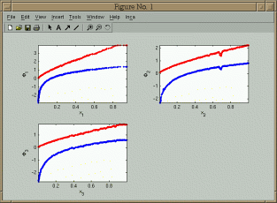
% Demonstration of how ACE finds logarithmic transformations
% Results in blue; red is exp(phi)

ll=500; % number of data points
dim=2;  % number of terms on right hand side
wl=5;   % width of smoothing kernel
oi=100; % maximum number of outer loop iterations
ii=10;  % maximum number of inner loop iterations
ocrit=10*eps; % numerical zeroes for convergence test
icrit=1e-4;
shol=1; % 1-> show outer loop convergence, 0-> do not
shil=0; % same for inner loop

x1=rand(ll,1); x2=rand(ll,1);
y=x1.*x2;
x=[y x1 x2]';

% call ace.m  ---------------------------------------------

[psi,phi]=ace(x,ll,dim,wl,oi,ii,ocrit,icrit,shol,shil);

% results -------------------------------------------------

psi

figure(1)
for d=1:dim+1;
subplot(2,2,d);
plot(x(d,:),phi(d,:),'.');
hold on;
plot(x(d,:),exp(phi(d,:)),'r.');
hold off;
axis tight;
xlabel(['x_{',num2str(d),'}']); ylabel(['\Phi_{',num2str(d),'}'])
end;

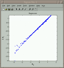
figure(2);
sum0=sum(phi(2:dim+1,:));
plot(phi(1,:),sum0,'.');
xlabel('\Phi_0'); ylabel('\Sigma \Phi_i'); title('Regression');
References
Breiman, L., Friedman, J. H.:
Estimating Optimal Transformations for Multiple regression
and Correlation, J. Am. Stat. Assoc., 80(391), 1985, 580-598.
Voss, H., Kurths, J.:
Reconstruction of nonlinear time delay models from data by
the use of optimal transformations, Phys. Lett. A, 234, 1997, 336-344,
doi:10.1016/S0375-9601(97)00598-7.