Differences between MI and MIGRAM

There is a minor difference between the results of the mutual information derived with mi and migram. The reason is that mi uses an algorithm as suggested by Roulston, M. S.: Estimating the errors on measured entropy and mutual information, Physica D, 125, 1999, which considers estimation errors (Px and Py are the probabilities of x and y, Pxy is the joint probability, and Nx, Ny and Nxy are the numbers of non-zero elements in Px, Py and Pxy):

Ix = -sum(Px * log(Px))
Iy = -sum(Py * log(Py))
Ixy = -sum(Pxy * log(Pxy))
Ixy_syserr = (Nx + Ny - Nxy - 1) / (2*length(x))
MI = Ix + Iy - Ixy + Ixy_syserr

In contrast, migram only uses the simple definition of mutual information:

Ix = -sum(Px * log(Px))
Iy = -sum(Py * log(Py))
Ixy = -sum(Pxy * log(Pxy))
MI = Ix + Iy - Ixy

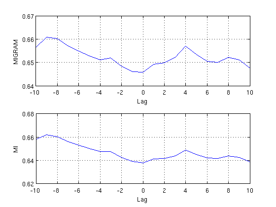
However, the trend in the results are quite similar.

Let us consider two oscillations

x = cos(0:.01:10*pi)';
y = sin(0:.01:10*pi)' + .1 * randn(length(x),1);

between which we will estimate the mutual information up to a lag of 10 steps.

Using migram we need to call this command with the arguments specifying the window length, which should be equal to the data length. In order to ensure that we use 10 bins we can also specify this argument.

m1 = migram(x,y,10,length(x),[],10);

The output m is a vector containing the mutual information between x and y from lag -10 up to +10 (hence, the length is 21)

m1'

ans =

  Columns 1 through 9

    0.6564    0.6608    0.6602    0.6570    0.6550    0.6528    0.6512    0.6519    0.6484

  Columns 10 through 18

    0.6461    0.6459    0.6492    0.6499    0.6522    0.6569    0.6534    0.6504    0.6501

  Columns 19 through 21

    0.6522    0.6510    0.6475

Using mi we again specify the number of bins and the maximal length (both 10).

m2 = mi(x,y,10,10);

The output is a 3-dimensional matrix, where the third dimension corresponds to the lag, and the first two dimensions to the first and second time series. E.g.,

squeeze(m2(1,1,:))'

ans =

  Columns 1 through 9

    2.1842    2.0405    1.9405    1.8567    1.7839    1.7198    1.6628    1.6122    1.5673

  Columns 10 through 11

    1.5278    1.4933

gives the auto mutual information of the first time series x for the lags 0:10, wheras

squeeze(m2(2,1,:))'

ans =

  Columns 1 through 9

    0.6378    0.6412    0.6419    0.6441    0.6489    0.6453    0.6423    0.6419    0.6440

  Columns 10 through 11

    0.6427    0.6388

gives the mutual information between x and y for lags 0:10. If we need the mutual information between x and y for lags -10:0, i.e. between y and x for lags 0:10, then we call

squeeze(m2(1,2,:))'

ans =

  Columns 1 through 9

    0.6378    0.6394    0.6427    0.6476    0.6478    0.6501    0.6531    0.6563    0.6604

  Columns 10 through 11

    0.6619    0.6582

Finally we compare the results derived with migram and mi in a plot. Note that we need to concatenate the components (1,2) and (2,1) of the results matrix derived with mi in order to get the mutual information of lags -10:10, and that the component (1,2) has to be flipped because it runs from 0:-10 but we need it to run from -10:0.

subplot(2,1,1)
plot(-10:10, m1)
grid on, xlabel('Lag'), ylabel('MIGRAM')
subplot(2,1,2)
plot(-10:10, [flipud(squeeze(m2(1,2,:))); squeeze(m2(2,1,2:end))])
grid on, xlabel('Lag'), ylabel('MI')