Import COPRA output and export ensemble data (time and proxy)

(N. Marwan, 2020-02-26)

Import COPRA output
The ensemble of time simulations
The ensemble of proxy values on a fixed time axis
Remark

Import COPRA output

The content of the COPRA output is stored in variable d. All variables can be accessed by d.VARNAME.

filename = 'BB-1_d13C_2015-03-18.mat';
load(filename)

The ensemble of time simulations

The ensemble of time simulations is in T_unc, starting with column 3. These times correspond to the depth values of each proxy measurement. The depth values are in d_prxy and also in the 1st column of T_unc.

depth = d.d_prxy;
t_ensemble = d.T_unc(:,3:end);

The ensemble of proxy values on a fixed time axis

The final time axis is 1st column in T_cert. The proxy values are in v_prxy and also in 2nd column of T_unc. These values have to be interpolated using the ensemble of age models in T_unc. We have M realizations.

t = d.T_cert(:,1);
proxy_ensemble = zeros(length(t), d.M);
for i = 1:d.M
   proxy_ensemble(:,i) = interp1(d.T_unc(:,i+2),d.v_prxy,t);
end

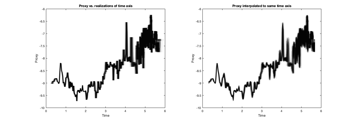
Remark

The ensemble of proxy values on a fixed time axis is a bit different from simply plotting the proxy values vs. the realizations of the time axis. In the first, the proxy values are interpolated to a new time axis, in the latter, the proxy values are untouched, but simply plotted at different time locations. The interpolated, therefore, look different.

subplot(1,2,1)
plot(t_ensemble(:,1:100),d.v_prxy,'color',[0 0 0 .1])
xlabel('Time'), ylabel('Proxy')
title('Proxy vs. realizations of time axis')

subplot(1,2,2)
plot(t, proxy_ensemble(:,1:100),'color',[0 0 0 .1])
xlabel('Time'), ylabel('Proxy')
title('Proxy interpolated to same time axis')

Import COPRA output and export ensemble data (time and proxy)

Contents